RF Power Amplifier Linearity: Understanding P1dB, IIP3 and OIP3

 The Relationship Between Key Linearity Parameters and Practical Measurement Methods

In RF power amplifier (PA) design and selection, linearity is one of the fundamental performance requirements. It directly affects the fidelity of an amplified signal and the level of unwanted distortion generated by the amplifier. Two of the most important parameters used to characterize PA linearity are P1dB (1 dB compression point) and IIP3/OIP3 (input/output third-order intercept point).

What is the relationship between these parameters? Can P1dB alone be used to evaluate amplifier linearity? And how should each parameter be measured in practice? This article explains the underlying concepts, engineering relationship, and common test methods in a practical way.

1. Understanding the Basics: What Do P1dB and IIP3/OIP3 Measure?

To understand the relationship between the two parameters, it is useful to first clarify what each one describes. An RF power amplifier ideally increases output power in proportion to input power while maintaining a constant gain. In the real world, however, active devices become increasingly nonlinear as the signal level rises. This nonlinearity eventually causes gain compression and generates unwanted spectral components.

1.1 P1dB: The Boundary of Linear Operation

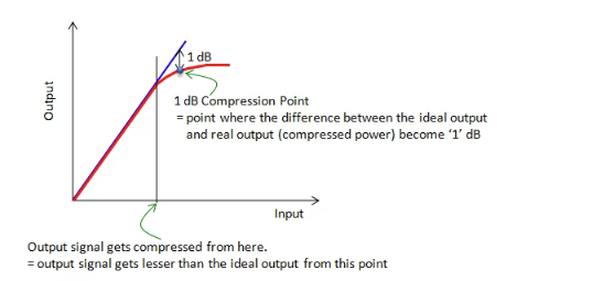
P1dB, or the 1 dB compression point, indicates the point at which an amplifier begins to depart significantly from its ideal linear gain. In the small-signal region, output power increases approximately linearly with input power, and the difference between output and input power represents the amplifier gain.

As input power continues to increase, the active devices inside the amplifier gradually approach saturation. The gain then begins to decrease. When the measured gain is 1 dB lower than the extrapolated small-signal linear gain, the corresponding output power is the output P1dB, while the corresponding input power is the input P1dB.

In practical terms, P1dB is a useful boundary for determining how much output power an amplifier can deliver before gain compression becomes significant. Operating substantially below P1dB generally provides more linear operation, while operation close to or beyond P1dB results in increasingly severe distortion.

P1dB should not be confused with saturated output power (Psat). Psat represents the region where further increases in input power produce little or no additional output power. The source article notes that Psat is typically about 3–4 dB higher than P1dB. In this sense, P1dB represents the point where compression becomes clearly measurable, while Psat represents a much deeper saturation condition.

1.2 IIP3 and OIP3: Indicators of Third-Order Linearity Performance

IIP3 (Input Third-Order Intercept Point) and OIP3 (Output Third-Order Intercept Point) characterize an amplifier’s tendency to generate third-order intermodulation distortion (IM3). This is particularly important in RF systems because third-order products can fall close to the desired signals and may be difficult to remove with filtering.

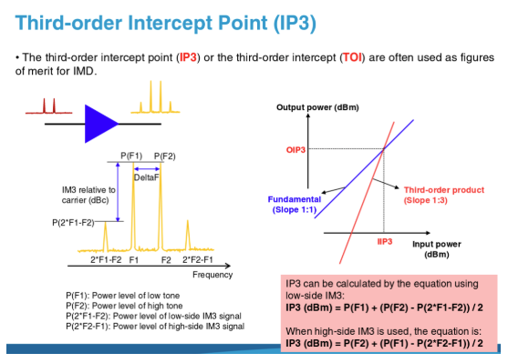
A common way to evaluate third-order distortion is the two-tone test. Two equal-amplitude tones at nearby frequencies, for example f1 = 1 GHz and f2 = 1.001 GHz, are applied to the amplifier. Because of device nonlinearity, the amplifier generates not only the two fundamental tones but also additional frequency components. The most important third-order products are 2f1 − f2 and 2f2 − f1.

If these products fall within or near the system’s operating band, they can degrade signal quality and increase interference. This is especially relevant to communication, RF test, radar, and other systems where spectral purity is important.

IIP3 and OIP3 are theoretical intercept points. If input power were continuously increased while the amplifier remained in its linear region, the fundamental output would increase with a slope of 1 dB/dB, while the third-order intermodulation products would increase at approximately 3 dB/dB. The extrapolated lines intersect at the third-order intercept point.

The physical intercept point is normally never reached in real operation because the amplifier enters compression and saturation before reaching that theoretical level. Therefore, IIP3/OIP3 should be understood as linearity indicators rather than practical operating power levels. A higher intercept point generally indicates stronger third-order distortion performance.

2. The Relationship Between P1dB and IIP3/OIP3

P1dB and IIP3/OIP3 both originate from the nonlinear behavior of the amplifier, but they describe different aspects of that behavior. They are complementary parameters rather than interchangeable specifications.

2.1 Common Physical Origin: Device Nonlinearity

Both gain compression and third-order intermodulation arise from the nonlinear transfer characteristics of the active devices inside the amplifier. As input power increases, nonlinearity first appears as deviation from ideal gain and then increasingly manifests itself through unwanted spectral products.

In simplified terms, P1dB focuses on when gain begins to compress, while IIP3/OIP3 focuses on the amplifier’s tendency to generate third-order distortion.

2.2 Practical Numerical Relationship

For many RF power amplifiers, OIP3 is often approximately 10–15 dB higher than P1dB as an engineering rule of thumb. This is an empirical relationship rather than a universal law, and the actual difference depends on amplifier architecture, device technology, bias conditions, frequency, output power level, and measurement method.

For example, if a PA has a P1dB of 30 dBm, an OIP3 in the approximate range of 40–45 dBm may be observed in some designs. The actual value must be verified by measurement rather than inferred solely from P1dB.

There is also a direct relationship between IIP3 and OIP3: OIP3 = IIP3 + G, where G is the amplifier’s small-signal or linear gain in dB. This allows engineers to convert between input- and output-referred intercept points.

2.3 Two Complementary Dimensions of Linearity

P1dB describes the usable output-power range before significant gain compression. IIP3/OIP3 describes the amplifier’s third-order distortion behavior within its linear operating region. Considering both gives a more complete picture of PA linearity.

• If P1dB is high but OIP3 is relatively low, the amplifier may provide substantial output power while generating comparatively strong third-order distortion at high drive levels.
• If P1dB is lower but OIP3 is high, the amplifier may provide excellent third-order linearity at lower output levels, which can be useful in applications where signal fidelity is prioritized.
• A design with both high P1dB and high OIP3 can combine high output capability with strong linearity, although achieving both may increase circuit complexity, power consumption, thermal requirements, and cost.

3. Is P1dB Alone Enough to Characterize PA Linearity?

No. P1dB is an important linearity specification, but it does not fully describe the type or magnitude of distortion generated by an amplifier.

Two amplifiers can have the same P1dB while exhibiting substantially different third-order intermodulation performance. For example, consider two PAs with a P1dB of 30 dBm and a linear gain of 20 dB. If PA A has an OIP3 of 45 dBm while PA B has an OIP3 of 40 dBm, their third-order distortion behavior under the same two-tone operating condition will be different even though their P1dB values are identical.

This illustrates why P1dB alone cannot distinguish all linearity characteristics. A PA can maintain gain to a relatively high output level yet still generate significant intermodulation products below its compression point.

For practical RF design, P1dB and IIP3/OIP3 should therefore be evaluated together with other relevant specifications, such as gain flatness, harmonic suppression, spurious emissions, noise figure, efficiency, and operating temperature, depending on the application.

4. Practical Measurement Guide: P1dB and IIP3/OIP3

The key principle of PA linearity testing is to minimize nonlinearity originating from the test setup itself. The measurement should reflect the true performance of the device under test (DUT), rather than distortion generated by the signal sources, cables, connectors, filters, or measurement instruments.

4.1 P1dB Measurement

Objective: determine the output power at which the amplifier gain is 1 dB below its extrapolated small-signal linear gain.

Method A: Manual Measurement with a Signal Generator and Spectrum Analyzer

Typical equipment includes an RF signal generator capable of producing a stable sinusoidal signal, a spectrum analyzer, the PA under test, RF cables, and an attenuator where necessary to protect the analyzer from excessive power.

Test procedure:

• Connect the test chain: RF signal generator → RF cable → DUT → attenuator (optional) → spectrum analyzer. Ensure proper grounding and secure RF connections.
• Establish the small-signal gain. Apply a low input level, for example −30 dBm, where the PA is clearly operating in its linear region. Record Pin1 and Pout1, then calculate G = Pout1 − Pin1.
• Increase the input power step by step. A 1 dB step can be used during the main sweep. Record Pin and Pout at each point and calculate the corresponding gain.
• Identify P1dB. When the measured gain is 1 dB lower than the initial linear gain, the corresponding output power is the output P1dB and the corresponding input level is the input P1dB.
• Correct for test-path loss. Measure or calibrate cable and attenuator losses so that the reported input and output power values accurately represent the DUT ports.
• 
  

For efficient testing, a larger step such as 2–3 dB can be used during the initial sweep. As the compression point is approached, reduce the step to approximately 0.5 dB for finer resolution.

Method B: Automated Measurement with a Vector Network Analyzer

A vector network analyzer with power-sweep gain-compression capability can automate the measurement and is useful for multi-frequency characterization.

• Select a swept-power gain-compression measurement and configure the amplifier’s operating frequency or multiple test frequencies.
• Set a power-sweep range that covers the expected P1dB point. The source article provides the example relationship PSTART = estimated P1dB − gain − 15 dB and PSTOP ≈ PSTART + 20 dB.
• Perform source-power calibration at each frequency point.
• Replace the calibration power sensor or probe with the DUT as required by the instrument procedure and run the measurement. The analyzer can then generate the input/output power curve and identify the 1 dB compression point.

4.2 IIP3/OIP3 Measurement: The Two-Tone Method

Objective: measure the fundamental output tones and third-order intermodulation products, then extrapolate the theoretical third-order intercept point while keeping the DUT in its linear region.

Typical equipment includes two RF signal generators (or a dual-tone source), a signal combiner, a high-dynamic-range spectrum analyzer, the DUT, RF cables, isolators, and low-pass filters. Isolators and filters help reduce unwanted interaction, harmonics, and nonlinearity generated by the test equipment itself.

Test procedure:

• Build the test chain: two RF sources → isolators → low-pass filters → signal combiner → DUT → isolator → low-pass filter → spectrum analyzer.
• Generate two closely spaced tones with equal amplitude, for example f1 = 1 GHz and f2 = 1.001 GHz. Keep the amplitude difference within approximately 0.1 dB for accurate measurement.
• Set the combined input level sufficiently below P1dB so that the amplifier remains in its linear region. The source article gives P1dB − 10 dB or more as a practical example.
• Measure the output power of the two fundamental tones, Pout1 and Pout2, and use their average as Pout when appropriate.
• Measure the two third-order products at 2f1 − f2 and 2f2 − f1 and use their average as PIM3.
• Calculate the power difference: ΔP = Pout − PIM3.
• Calculate OIP3: OIP3 = Pout + ΔP/2.
• Calculate IIP3: IIP3 = OIP3 − G, where G is the amplifier’s linear gain.
• Repeat the measurement several times at different input levels while staying in the linear region, then average the results to reduce measurement uncertainty.

A spectrum analyzer must have sufficient dynamic range to resolve weak IM3 products, which can be tens of dB below the fundamental tones. The test environment should also be well controlled to minimize external electromagnetic interference.

5. Key Takeaways for RF Power Amplifier Design

P1dB and IIP3/OIP3 represent two different but complementary dimensions of RF power amplifier linearity. P1dB indicates the onset of significant gain compression and helps define the amplifier’s usable output-power range. IIP3/OIP3 provides information about third-order intermodulation behavior and signal fidelity within the linear operating region.

For applications such as wireless communications, RF test equipment, radar, satellite communications, and professional radio systems, relying on a single linearity parameter may lead to an incomplete assessment. The appropriate combination of P1dB, OIP3/IIP3, gain, efficiency, harmonic performance, and thermal characteristics should be selected according to the system requirements.

In simple terms: P1dB answers the question, “How much output power can the amplifier deliver before significant gain compression?” IIP3/OIP3 helps answer, “How well can the amplifier suppress third-order distortion while operating in its linear region?” Together, these parameters provide a much more complete understanding of RF PA linearity.

6. Custom RF Power Amplifier & OEM/ODM Support

For OEM and ODM projects, RF power amplifier linearity should be optimized as part of the complete amplifier architecture rather than treated as a single isolated specification. Frequency range, output power, gain, P1dB, OIP3, harmonic suppression, input/output VSWR, efficiency, thermal management, control interface, mechanical enclosure, and operating environment can all influence the final design.

ZR Hi-Tech provides customized RF and microwave amplifier solutions for application-specific requirements. Customization can cover frequency bands, output power, gain, package and mechanical dimensions, thermal design, control interfaces, connectors, and other electrical specifications. For projects with defined P1dB or IIP3/OIP3 targets, engineering evaluation can be performed based on the required operating conditions and test criteria.

If you are developing an RF power amplifier for communications, radar, RF test, satellite, EW, industrial, or other high-performance applications, share your target frequency, output power, gain, linearity requirements, and mechanical constraints with our engineering team. 

We can evaluate the requirements and propose a suitable customized RF amplifier solution.

Contact: info@zrhitech.com | www.zrhitech.com